Tile Scheduling
Motivating the issue
A matrix multiply is embarrassingly parallel. Each output tile can be computed independently. There are no data dependencies, no synchronization, and no ordering constraints. This is a kernel that can run at about 1.05x the speed of CuBLAS at M=N=K=8192. Yet, when we naively order our tiles, don't use a persistent kernel, and don't use TMA multicast, our performance precipitously drops by around 20%. Though a matrix multiply may be embarrassingly parallel, not only when but how you access data certainly does matter.
The tiles themselves, thus, are compute-independent but memory-dependent. They share input data. Tile (0, 3) and tile (1, 3) both read the same B column stripe. Whether that stripe is in L2 or DRAM depends on whether someone recently read it, which depends on visit order.
The GPU has a shared cache but it doesn't have a shared scheduler. L2 may be shared across all SMs, but the runtime assigns tiles to SMs without thinking about data sharing. This necessitates having to encode the sharing pattern into the tile-to-SM mapping yourself, which motivates needing a "smart" tile scheduler.
But even a smart tile ordering only defines which tile each cluster computes. Without persistence, each cluster computes one tile and exits. The next cluster to land on that SM would need to re-warm L2 from scratch. Persistence keeps a small set of clusters alive, each processing a sequence of related tiles, whereby the data warmed by one tile is still in L2 when that same SM starts its next tile.
Yet even with persistence and a smart tile ordering, if we think back to our tiles (0, 3) and (1, 3), each would still need to issue separate TMA loads to pull the same shared B stripe from L2 into their respective SMEMs. With CTA multicasting those two separate TMA transactions are collapsed into one and data is broadcast directly to both CTAs simultaneously.
Some numbers
On an H100, we have 50MB of shared L2 cache and 256KB of combined shared memory and L1 cache with only about 228KB usable. For the sake of easy math, let's assume our data is in bfloat16 and we have a tile shape of (128, 128) => 128 x 128 x 2 bytes == 32KB per tile and M=N=K=8192. This means we have an output grid of 64 x 64 == 4096 tiles. A single stripe of matrix A is 128 * 8192 * 2 bytes == 2MB. B is the same size. Per K-step (k-tile size == (128, 128)) for both A and B (2 x (128 x 128 x 2 bytes) == 64KB). We can fit 50MB / 2 MB == 25 A or B stripes in L2 at once. Cumulatively, A and B take up 2 x (8192 x 8192 x 2 bytes) == 256 MB.
Lastly, an H100 SXM has 132 SMs. With a cluster shape of (1,1,1) (i.e. one CTA per cluster), one wave is 132 clusters launched simultaneously on each SM. So, in total we'll execute math.ceil(4096 / 132) == 32 waves or 32 batches of 132 independently running matrix multiplies (the last batch will only be partially full with 4096 - 132 * 31 == 4 active clusters).
Tile ordering
So tile order matters, but why? Let's think through what data from A and B will be loaded in our naive scenario. In wave 1, we have 132 tiles, and naively tiling from top to bottom, left to right, has us computing output tiles for each column of the first two output rows and the first four columns of the third output row.
This equates to 3 * 2MB = 6MB from A and 64 * 2MB = 128MB from B. So, necessarily, as we progress through each of our 128 k-steps, eventually the initial A and B tiles from earlier k-steps will be evicted in favor of the current k-step's data needs. This implies that come the next wave, we will need to reload from global memory all of B. Furthermore, each subsequent k-step sees 3 distinct A chunks loaded and 64 B chunks loaded (67 * 32KB = 2.14MB of data load from global memory per k-step).
The question is can we do better?
We know that a full stripe of A or B in our scenario is 2MB and that at some point A needs to stripe across each stripe of B. So, what if we only computed the first, say, 12 stripes of B? That would mean we'd need to load ceil(132 / 12) == 11 stripes from A as each stripe of A could reuse each stripe of B 12 times. This implies we need to load (12 + 11) * 32KB = 1.056MB per k-step and 12 * 2MB + 11 * 2MB = 46MB in total from global memory across the entire first wave. But on the subsequent wave, our entire 12 stripes of B should still be resident in L2 cache and we'd only need to load 11 * 2MB = 22MB of A. Huge bandwidth savings!
CTA swizzling and Hilbert curves both try to optimize for this exact problem of maximizing data reuse across the cache hierarchy and minimizing total memory traffic.
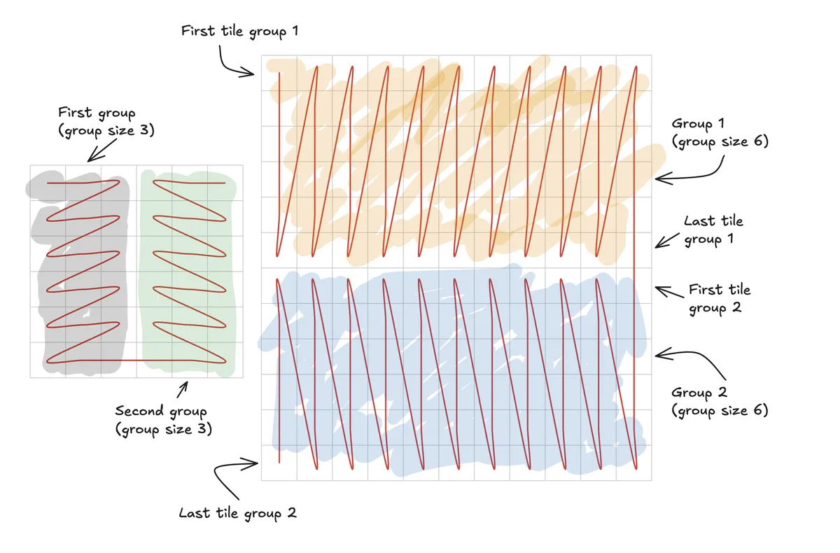
CTA swizzling aims to ensure that each group of tiles share proximity, though any two consecutive block indices need not necessarily share either an A or B stripe. The idea is the group collectively reuse stripes of A and B. CTA swizzling utilizes serpentine ordering, whereby the subsequent group reverses the direction of the current group and starts from the opposite side. As you can see below, both CTA swizzling itself and serpentine ordering help to maximize L2 cache reuse.
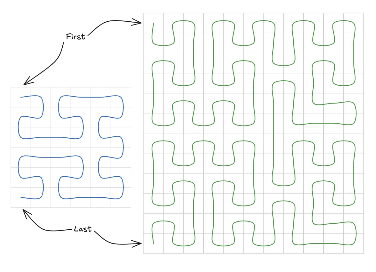
Hilbert curves allow you to fill some space (i.e. our grid of tiles) with a continuous path through those tiles. Compared to CTA swizzling, no care has to be put towards the remainder of tiles if some group doesn't fit across some dimension because we are now space filling as opposed to ensuring some clustering or grouping of tiles is always proximal to one another.
When we compare the runtimes (non-persistent kernel, (128, 128) tile shape, (1,1,1) cluster shape), we see:
| Ordering | Group Size | ms |
|---|---|---|
| Naive raster | — | 2.116 |
| Hilbert | — | 1.880 |
| Swizzle (online) | 8 | 1.952 |
| Swizzle (online) | 12 | 1.944 |
| Swizzle (online) | 16 | 1.933 |
| Swizzle (online) | 20 | 1.908 |
| Swizzle (online) | 24 | 1.907 |
| Swizzle (online) | 28 | 1.906 |
| Swizzle (online) | 32 | 1.928 |
| Swizzle (offline) | 8 | 1.946 |
| Swizzle (offline) | 12 | 1.933 |
| Swizzle (offline) | 16 | 1.914 |
| Swizzle (offline) | 20 | 1.911 |
| Swizzle (offline) | 24 | 1.897 |
| Swizzle (offline) | 28 | 1.912 |
| Swizzle (offline) | 32 | 1.953 |
Note that "online" swizzle computes each tile's coordinates arithmetically on the device. "Offline" swizzle and Hilbert both precompute a lookup table on the host, mapping each linear tile index to its 2D coordinates, then pass the look-up table to the kernel. Since offline swizzle and Hilbert share the exact same kernel code path, the performance difference between them is purely a property of the traversal pattern, not the instruction mix.
The group size sweep also reveals a fundamental tradeoff, namely that larger groups improve B-column reuse (more tiles share the same B stripe) but degrade A-row locality (the group spans more rows of A). The sweet spot around group size of 24 balances these competing effects. Hilbert curves avoid this tradeoff entirely. The curve inherently balances both M and N reuse by construction, which is why it beats the best swizzle group size without any tuning.
For our setup, there's a sweet spot near group size of 24 for both swizzle variants. The best swizzle configs come to within around 1% of using Hilbert curves, but Hilbert still beats CTA swizzling (and is over 11% faster than naive rastering!) and requires no group size tuning.
With a baseline ncu profiling we see:
| Metric | Naive Raster | Hilbert | Swizzle (online, gs=12) |
|---|---|---|---|
| Duration | 2.06 ms | 1.89 ms | 1.94 ms |
| L2 Hit Rate | 51.77% | 75.44% | 77.96% |
| DRAM Throughput | 82.95% | 33.59% | 31.65% |
| L2 Cache Throughput | 97.66% | 88.25% | 92.01% |
| Avg L2 Active Cycles | 3,619,869 | 3,173,514 | 3,297,835 |
From these metrics alone, the story isn't entirely clear. CTA swizzling has a better L2 hit rate and lower DRAM throughput, which would suggest better L2 reuse. Yet Hilbert is faster. The clue is in the L2 cache throughput and active cycles. Hilbert's L2 is less busy, suggesting it handles less total L2 traffic.
Looking more deeply into L2 traffic, the story becomes clearer:
| Metric | Naive Raster | Hilbert | Swizzle (gs=12) |
|---|---|---|---|
| L2 Total Sectors | 605,277,174 | 516,214,595 | 545,137,175 |
| L2 Lookup Hits | 306,263,218 | 388,933,078 | 422,633,862 |
| L2 Lookup Misses | 293,533,349 | 121,083,552 | 118,394,239 |
| L2 Hit Rate (computed) | 51.1% | 76.3% | 78.1% |
Swizzling has a better L2 hit rate and fewer absolute misses, but Hilbert sends ~29M fewer total sectors through L2 (516M vs 545M). A sector is the fundamental unit of data transfer in our memory hierarchy and equals 32 bytes. Each sector read, either on hit or miss, consumes L2 bandwidth. And with L2 already running at nearly 90% of peak throughput, those extra 29M sectors from swizzling create queuing and backpressure, which slows the kernel down.
Fewer total sectors is a result of the different traversal patterns. Within a swizzle group, consecutive tiles walk along the raster dimension (down M rows and across group size columns or across N columns and down group size rows depending on raster order). As you can see in the swizzle image above, every group_size number of tiles, the path jumps resulting in two consecutive tiles that may share neither a row nor a column. Any A stripes that were warm from the previous usage could go cold before the traversal returns to that data. The hilbert curve has no such jumps because each consecutive pair of tiles is adjacent on the 2d grid, allowing for sharing of either of row or column.
At a high level, Hilbert wastes less time re-loading data it already had. In Hilbert, data is consumed before it can be evicted, which avoids re-fetches that inflate the swizzle's total L2 traffic. So swizzle is “more cache-hit efficient” as a ratio, but Hilbert creates less L2 work overall. Since L2 is already near saturation, fewer total L2 sectors beats a slightly higher hit rate.
Clearly, losing L2 residency hurts. Tile ordering gives us locality within a wave, but persistence gives us locality across work assigned to the same resident CTA. Without persistence, every wave boundary is a potential cold start, where the next CTA that lands on an SM may correspond to a tile with poor reuse of the data that SM just helped bring into L2.
Persistence
In a non-persistent kernel, each CTA computes one tile and exits. The remaining CTAs are already part of the launched grid, so the GPU simply keeps filling SMs with pending CTAs. But that scheduling is not cache-aware. The next CTA that lands on a given SM is not selected because it reuses the data that SM just helped pull into L2. Persistence gives you a way to make that “next tile” decision inside the kernel, where your tile scheduler can preserve locality across the sequence of tiles handled by the same resident CTA.
Persistent kernels break down into effectively two shapes, static and dynamic. Static persistent kernels means tiles get assigned using fixed math at launch. For instance, SM 0 will always take tiles 0, 132, 264, etc. Dynamic persistent kernels might use some global atomic counter where SMs grab the next available work index.
Now with persistence, comparing runtimes we see:
| Ordering | Group Size | Static (ms) | Dynamic (ms) |
|---|---|---|---|
| Naive raster | — | 2.284 | 2.129 |
| Hilbert | — | 2.189 | 1.862 |
| Swizzle (online) | 8 | 2.062 | 1.914 |
| Swizzle (online) | 12 | 2.099 | 1.898 |
| Swizzle (online) | 16 | 2.087 | 1.880 |
| Swizzle (online) | 20 | 2.095 | 1.854 |
| Swizzle (online) | 24 | 2.089 | 1.847 |
| Swizzle (online) | 28 | 2.104 | 1.856 |
| Swizzle (online) | 32 | 2.137 | 1.904 |
| Swizzle (offline) | 8 | 2.054 | 1.917 |
| Swizzle (offline) | 12 | 2.103 | 1.908 |
| Swizzle (offline) | 16 | 2.088 | 1.879 |
| Swizzle (offline) | 20 | 2.089 | 1.860 |
| Swizzle (offline) | 24 | 2.102 | 1.846 |
| Swizzle (offline) | 28 | 2.105 | 1.860 |
| Swizzle (offline) | 32 | 2.154 | 1.890 |
And our same baseline NCU profiling:
| Metric | Naive Raster | Hilbert | Swizzle (online, gs=24) |
|---|---|---|---|
| Duration | 2.08 ms | 1.86 ms | 1.84 ms |
| L2 Hit Rate | 51.00% | 80.44% | 66.23% |
| DRAM Throughput | 85.11% | 34.34% | 55.09% |
| L2 Cache Throughput | 95.93% | 92.75% | 93.64% |
| Avg L2 Active Cycles | 3,465,806 | 3,219,650 | 3,130,297 |
And more deeply into L2.
| Metric | Naive Raster | Hilbert | Swizzle (gs=24) |
|---|---|---|---|
| L2 Total Sectors | 601,690,715 | 530,109,580 | 542,488,980 |
| L2 Lookup Hits | 311,523,661 | 417,308,590 | 378,907,597 |
| L2 Lookup Misses | 307,231,020 | 116,238,580 | 173,166,763 |
| L2 Hit Rate (computed) | 50.3% | 78.2% | 68.6% |
Interesting! Hilbert had fewer total L2 sectors, more L2 hits, and fewer L2 misses, but swizzle had fewer L2 active cycles and is now slightly faster than the best Hilbert config.
How could this be?
In a standard, non-persistent kernel, the GPUs hardware block scheduler will assign a wave of 132 CTAs to the 132 SMs. When some SM finishes its assigned tile, that block exits. This lifecycle creates a natural "pause" in the memory request stream. You have teardown and setup overhead (cleaning/setting up registers, (de)allocating shared memory, etc), prologue instructions (initializing barriers, etc), and temporal jitter (CTAs finishing at different times cause staggered entry and exit). This creates a sort of "air" into the memory subsystem.
In the persistent case, these gaps are removed and the memory system is forced to run at its limit. Once some SM finishes its epilogue, the warp loops around, grabs its next tile index, and starts issuing memory requests. This is the reason why (as we spoke about above where there was a "tail" in last wave of clusters), the tail effect is drastically reduced.
Let's take a look at the sort of geometry that will inform which next tile some CTA will be assigned in both the swizzle and Hilbert cases.
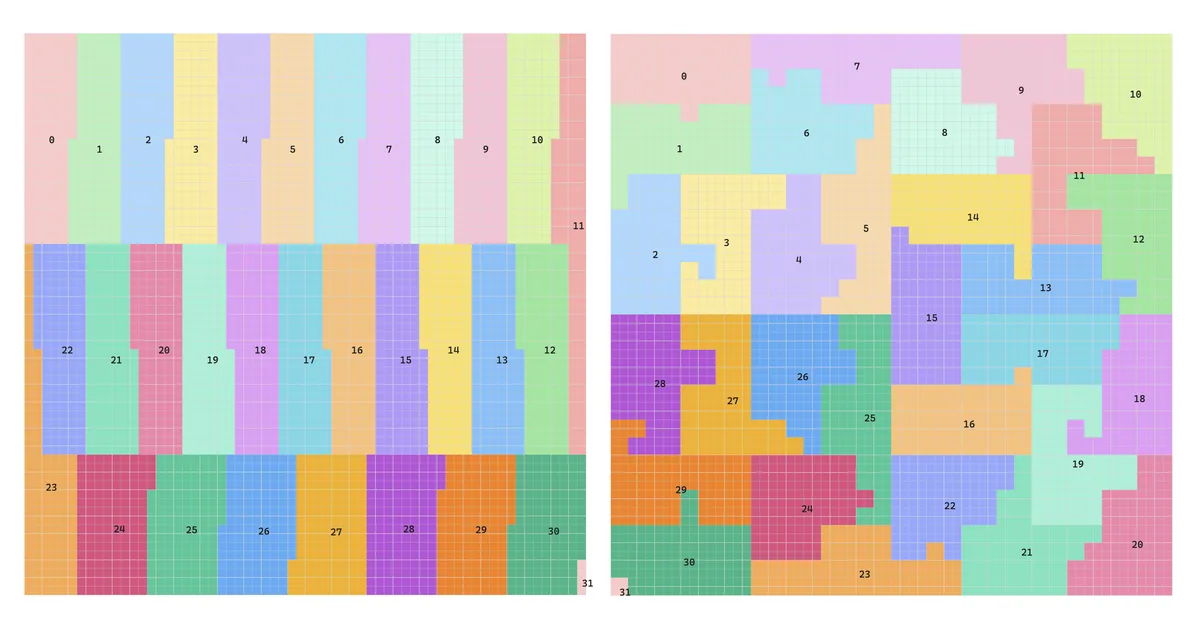
The question is why does the swizzle geometry appear to play less nicely with L2 than Hilbert yet allow the kernel to run faster. To answer this, we take a turn into GPU internals.
Between each SM and L2 sits a crossbar. L2 itself is split first into some smaller number of partitions, then within those partitions, split into channels, where each channel owns some portion of L2 cache. Each physical L2 partition has its own crossbar, which mediates access between an SM and an arbitrary L2 channel.
Furthermore, each SM is physically mapped to a specific partition. The latency between some SM and a given L2 channel, which resides in the same partition that the SM is mapped to, is equal. Crucially, though, if some chunk of L2 data that an SM accesses is not within its own partition, the request gets routed across the crossbar bridge so a different crossbar can handle that request. This incurs overhead.
Moreover, how some physical address gets mapped to a channel, and L2 cacheline, is through a black-box hashing function. The function itself attempts to ensure that physical VRAM addresses get mapped evenly across channels to maximize throughput, as simultaneous access to the same channel can cause L2 contention due to the L2 cache controller only being able to handle a limited number of requests per cycle.
Much of that information can be found here and here.
So, how does this information rectify our confusion?
If we take a look at an ncu metric called smsp__warp_issue_stalled_long_scoreboard_per_warp_active.pct, we see that for Hilbert it is 60% and for swizzle 55%. SMSP stands for streaming multiprocessor sub-partition. The metric is to say that the SMSP's warp scheduler looked at its pool of active warps during some clock cycle to issue an instruction, but couldn't find a single warp ready to fire because they were waiting for some memory operation to complete. Long scoreboard stalls specifically speak to the warp waiting on some global memory operation and indicate that both latency hiding has collapsed and execution cores are sitting idle.
Looking at a different metric called smsp__warp_issue_stalled_mio_throttle_per_warp_active.pct, we see that for Hilbert it is 44% and for swizzling 58%. MIO (memory input/output) throttling occurs when some kernel is making memory requests to its crossbar faster than the hardware can handle them. Once the queue hits maximum capacity, backpressure gets exerted on the warp scheduler and thus pauses any warp trying to issue another memory instruction. This gets logged as a MIO throttle stall. In conjunction with the long scoreboard metric, we can ascertain that in the Hilbert case, because the warps are constantly waiting at the L2 traffic jam, they rarely get to execute new memory instructions. Thus the queue stays emptier for longer unlike the swizzle kernel.
These metrics alone are enough to point us towards an answer to our problem. The Hilbert curves force CTAs to process data in a highly localized and tightly bunched 2d cluster, and the concurrent SMs request physical memory addresses that are highly correlated. This high correlation seems to break down the hashing function, which outputs similar channels for a given clustering of tiles. This similarity in channel destination allows for great L2 hit rates as we see. However, it not only causes major contention on single channels but also forces SMs to cross the crossbar bridge for each memory transaction, which leaves the warps stalled for longer. On the other hand, swizzling with a certain group size seems to allow us to spread our data accesses more uniformly across more physical L2 slices, which results in the warps stalled for less time and thus greater latency hiding.
CTA Multicasting
Given the hardware realities we're constrained by, and the gemm that we're running, it is then natural to wonder about two consecutive CTAs issuing loads for the same B tile. Say these CTAs are on SM0 and SM1 and issue loads for some chunk of B at the same time. They'll make requests that go through the same crossbar to the same L2 channel to potentially wait in a queue in order to load the same data. Thinking about all the adjacent CTAs that may be doing just this, we realize how greatly we might be able to reduce our L2 contention if SMs could cooperate.
CTA clusters and multicast give us a means to do just this. If related CTAs are placed in the same cluster (similarly to how we group our tiles), one TMA load can multicast a tile to multiple CTAs, potentially on different SMs.
We note that the shape of our cluster should either inform or be informed by both the raster order of our kernel and the group size of our swizzle.
Looking at some metrics when using a cluster of shape (2,1,1):
| Ordering | Duration | L2 Sectors | Long Scoreboard | MIO throttle |
|---|---|---|---|---|
| Hilbert, no multicast | 1.88 ms | 532.9M | 60.18% | 0.44% |
| Hilbert, multicast | 1.57 ms | 441.9M | 38.85% | 0.82% |
| Swizzle, no multicast | 1.83 ms | 539.0M | 55.42% | 0.58% |
| Swizzle, multicast | 1.39 ms | 364.7M | 11.23% | 5.69% |
Clustering reduces the amount of repeated work the memory system has to do as we can see in the L2 sectors count. The real wins show up in our long scoreboard metric. We've greatly reduced our L2 congestion, so less often is some warp scheduler waiting on memory operations to complete.
Conclusion
While matrix multiplication is compute-independent, achieving peak performance requires orchestrating data access to perfectly match the intricate layout of the GPU memory subsystem. As the metrics show, maximizing efficiency is a delicate balancing act between maintaining raw cache locality and distributing traffic uniformly across L2 channels to prevent hardware level channel contention. Ultimately, pairing an intelligent tile scheduler with persistent kernels and CTA multicasting is part of what goes into making highly performant kernels.